The following is a conversion of my bachelor’s degree senior thesis. Not all of the conversions to a web format work properly. You can see the original LaTeX version here
Acknowledgements
I’d like to begin by acknowledging that this research project took place during the COVID-19 pandemic. I want to thank the healthcare workers, essential workers, professors, and the larger UCI community for all the work and dedication they provided during the transition to remote instruction.
I want to personally extend my thanks to Professor Manoj Kaplinghat who, not only accepted me into his research group but also provided constant and invaluable insight and advice throughout my research project. I consistently drew from his knowledge and expertise in the field, without which, this would not have been possible. I would also like to thank all the other members of the research group, most of all Alex Lazar who provided assistance and guidance and made himself available for all manner of questions. I want to also thank Professor Mariangela Lisanti and the rest of the self-interacting dark matter research group at Princeton for their collaboration and insight. Lastly, I’d like to thank my family and friends who supported and encouraged me throughout the process, especially when I lost confidence.
Abstract
Particle simulations are at the heart of the search for dark matter. The ability to quickly and accurately resolve dark matter subhalos–regions of virialized dark matter gravitationally bound to larger host halos–can help investigate regions of parameter space quickly and efficiently. We explore the self-interacting dark matter (SIDM) and a more efficient method to incorporate interactions between simulated dark matter subhalos and their host, represented by an analytic potential. This approach could greatly reduce the computational power required to incorporate such host-subhalo interactions while maintaining high accuracy. We conclude by incorporating these modifications into the codebase of the popular multi-physics and cosmological simulation suite GIZMO.
Introduction
Historical Observations
In 1933, Swiss Astrophysicist Fritz Zwicky published a paper of his findings studying the Coma Cluster, a large galaxy cluster located in the constellation Coma Berenices. Zwicky used spectroscopy to calculate the velocities of galaxies in the cluster. He then used the cluster’s overall luminosity to estimate its mass, and therefore its escape velocity. When comparing the two, Zwicky made a startling discovery. He found that the galaxies in the cluster had velocities far too high to be gravitationally bound by the visible mass of the cluster alone.
This left one of two possibilities: either Zwicky miscalculated the galaxy velocities, or he miscalculated the cluster’s escape velocity. In his paper, Zwicky concluded the latter and estimated the ratio of non-visible matter to visible matter in the cluster was 400:1. While this would turn out to be highly overestimated, the core conclusion was still valid: there is far more matter in the Universe that we cannot see, than matter that we can.
Zwicky’s conclusions were not immediately taken seriously, and it wouldn’t be until much later and with much more evidence that the theory of dark matter became widely accepted. One of the more compelling pieces of evidence for the existence of dark matter came from the analysis of galaxy rotation curves in the 1970s.
\subsection{Galaxy rotation curves} To understand how shocking the results of galaxy rotation curve analyses were, let’s first examine the simple Newtonian case, excluding dark matter. Assuming the only force acting on stellar bodies is the gravitational force (not a bad approximation) we can equate the centripetal acceleration to the gravitation acceleration as follows: $$ \frac{v^2}{r} = \frac{GM(r)}{r^2} $$ Where $G$ is the gravitational constant, $v$ is the body’s tangential velocity, and $M(r)$ is the galaxy’s mass interior to the radius $r$. Now solving for the velocity $v$, we find: $$ v(r) = \sqrt{\frac{GM(r)}{r}} $$ Looking at our solar system, the mass of the sun dominates the mass of the solar system, so we can make the approximation $M(r) \approx M_{\odot}$ for all planetary bodies. This implies that the further a body is from the sun, the slower its velocity around the sun. This is a slightly modified version of Kepler’s third law and is well corroborated by everything we see in our neighborhood.
So, it was assumed that a similar relationship likely held for galaxies, since the bulk of the baryonic matter (the matter which interacts with light) is concentrated at the center of the galaxy–much like in the solar system–thus we would expect a velocity decay roughly proportional to $r^{-\frac{1}{2}}$.
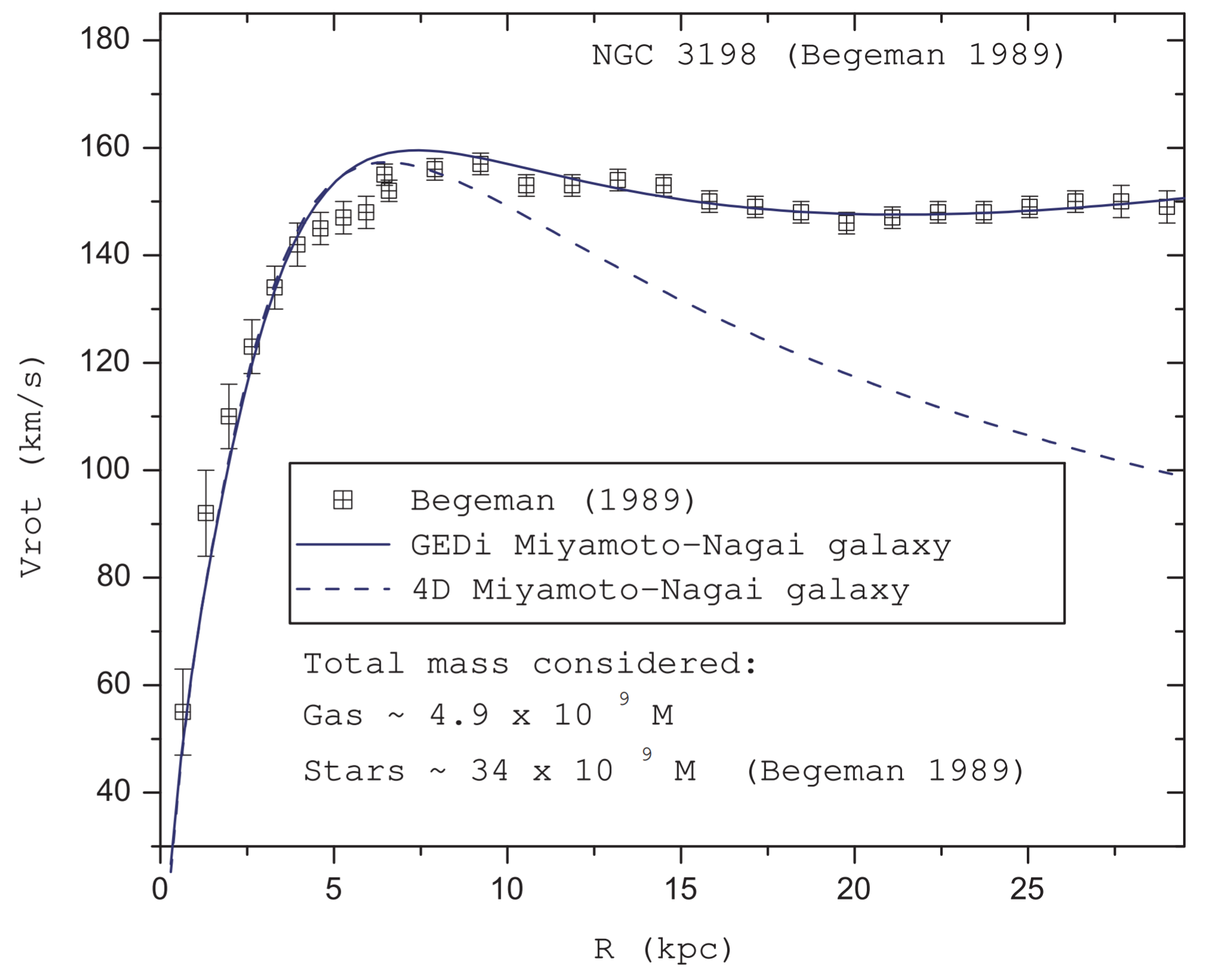
However, this assumption is contradicted by the observed rotation curves of galaxies, as seen in figure 1. Rotation curves show that rather than decaying with increasing radius, the tangential velocities of gravitationally bound matter in galaxies remain mostly constant regardless of their distance from the galactic center \cite{rubin_rotation_1970}.
Several solutions were proposed to reconcile decaying velocity curves–as predicted by Newtonian dynamics–with the constant ones observed. One theory, proposed by Israeli Physicist Mordehai Milgrom was coined Modified Newtonian Dynamics. MOND suggests that Newton’s Laws function differently on galactic scales than on smaller, solar system scales. However, even by modifying Netwon’s laws, MOND cannot account for all the mass required to explain certain galaxy clusters [McGaugh]. However, even if this aspect of the theory were resolved, MOND would still fail to compete with the explanatory power of dark matter. The dark matter model, by contrast, is well supported by weak and strong lensing, Big Bang nucleosynthesis, and the large-scale structure of the Universe, among others.
The inclusion of dark matter reconciles the apparent tension between Newtonian dynamics and observed rotation curves by changing our assumptions about the mass profiles of galaxies. Constraints on the amount of dark matter in the Universe put its prevalence at approximately 5 times more abundant than baryonic matter. These constraints increase the amount of matter in galaxies sufficiently enough to reproduce the rotation curves as given by the data.
Dark Matter Candidates
If we take seriously the theory of dark matter, a key property of all prospective dark matter candidates is that they do not interact–or interact very weakly–with light. A more technical description is that any prospective dark matter candidate must have a very small interaction cross section with photons–the electromagnetic gauge boson. However, this still leaves many possible dark matter candidates.
Some possible dark matter candidates live comfortably in unexplored parameter space, others are consequences of theories presented as solutions to unrelated problems but also make compelling dark matter candidates, but none of them have been constrained well enough, or observed definitively enough to be the conclusive front runner in the field. The field of dark matter candidates is very much still evolving and undergoing active research.
WIMPs
WIMPs or weakly-interacting massive particles are theoretical subatomic particles with a mass around $m_w \sim$ 10 GeV- 10 TeV. WIMPs are one of the most studied dark matter candidates, they are a consequence of theories in particle physics and hold the promise of being directly observable on earth. Additionally, the theories which predict the existence of WIMPs also constrain their relic density to a value consistent with that required of dark matter, this fact is often referred to as the WIMP miracle.
The early Universe was a much denser and much hotter place. Regions of space contained particles in sufficient quantities and at high enough temperatures to allow for the creation of heavier particles from lighter ones due to interactions. Likewise heavier particles could undergo pair production, creating lighter particles. For a period of time, these two processes occurred in relatively equal amounts. However, as the Universe expanded and cooled this thermal equilibrium broke down, and there ceased to be enough particles to allow for the creation of heavier particles from the interactions of two lighter ones. As a result, the abundance of these heavier particles has remained constant since the early Universe. This gives rise to a useful quantity in describing dark matter candidates: relic density. A particle’s relic density is its density just prior to freeze-out.
Another tantalizing aspect of WIMPs is that they can in theory be detected on earth either indirectly or directly. This is a rarity as all observational data of dark matter currently only comes from its gravitational influence. In order to detect WIMPs we first assume they annihilate with one another, producing particles in the standard model. It may in turn be possible to detect these produced particles giving indirect evidence for the existence of WIMPs.
Another possible detection method is direct detection. Since we expect these particles to interact only via the weak force, their interaction rate would be exceedingly low making them very difficult to detect and differentiate from background noise in the detector. So WIMP detectors including DEAP, ZEPLIN-III, and XENON are placed very deep underground and great care is taken to eliminate all other contaminating sources. They use large vats of Nobel gases supercooled to liquids as their detection mediums. In theory, if a stray WIMP were to pass through the detector at just the right place, it could interact with the nuclei of the Nobel gas, exciting it and causing the emission of a photon, which in turn could be seen by the detector.
However as of yet, despite an extensive effort by particle physicists the world over, WIMPs have never been detected. Casting doubt on their existence and constraining them to ever-smaller regions of parameter space.
MACHOs
Another dark matter candidate are massive astrophysical compact halo objects, also called MACHOs. These are astrophysical objects which are typically made of baryonic matter, but which have extremely high mass-to-luminosity ratios. These objects could contribute substantially to the mass of their host galaxy while remaining very difficult to detect and thus difficult to have their mass accounted for with observations.
One possible MACHO candidate is black holes. Isolated black holes–absent of an accretion disk–do not emit any light and could exist in far greater numbers than currently predicted. If true this would certainly account for some of the missing mass attributed to dark matter. Other possibilities include brown dwarfs: massive gas-giant-like objects, just shy of undergoing hydrogen fusion in their cores. These ‘super Jupiter’ objects are very massive but produce very little light of their own. Another candidate is neutron stars: the cores of dead stars not large enough to explode in supernovae. Since Neutron stars are extremely dense and are not actively undergoing fusion, they have low luminosity, but still account for the majority of the mass of the stars they were formed from.
MACHOs are compelling since they are already known to exist, and have low enough luminosities to remain mostly unaccounted for in mass calculations. Since we know they exist, they likely account for some percentage of the dark matter in the Universe; but studies have cast doubt on their ability to account for all of it. One such study found that only $10-40%$ of the Milky Way’s dark matter halo could come from MACHOs.
Another roadblock for MACHOs is the fact that we know that the majority of dark matter must come from non-baryonic sources, and while MACHOs can be non-baryonic, eliminating the baryonic MACHO sources reduces the effectiveness of the argument made previously regarding MACHOs coming from well-understood sources.
Axions
Axions are a theoretical subatomic particle, whose existence is implied by a field first proposed by Helen Quinn and Roberto Peccei in 1977, as a solution to the strong CP problem. A simplified example of the strong CP problem can be seen as follows:
Neutrons are composite particles, made of three quarks: one up and two down quarks. Each of these quarks carries their own electric charge, but combine to generate a net zero charge. For a moment consider another such composite structure, say $H_2O$. $H_2O$ is likewise electrically neutral but comprised of non-neutral atoms. This gives rise to water being polarized, which is to say it has a measurable electric dipole moment. We would expect the same to be true of the neutron. However, this is not the case. Instead, the neutron appears to have an electric dipole moment far lower than its theoretical value. Specifically, its electric dipole moment has been constrained on the order of $d_e < 10^{-27}e; \text{cm}$, while theory puts their EDM at $d_e \approx 10^{-16}e\ \text{cm}$.
And while the axion was first proposed as a consequence of a new field proposed to solve the above problem, they also have properties that would make them a compelling candidate for dark matter. Even though axions would need to be extremely low mass, with a lower bound of approximately $10^{-5}eV$ and an upper bound of order $10^{-3}eV$, they would need to be extremely numerous. Models suggest axions would likely have very low interaction cross sections for the strong and weak forces and carry no charge for interaction via the electromagnetic force.
$\Lambda$CDM
Before discussing self-interacting dark matter–which will be the subject of the remainder of this paper–we first need to discuss the model which it inherits (albeit with some key differences).
$\Lambda$CDM is a framework that is considered “the standard model of big bang cosmology.” The model began to take shape in the early 1960s and by the early 1990s, it includes an explanation for the expanding rate of the Universe, in the form of dark energy (the $\Lambda$ in its name). Additionally, the model explains the anisotropy of the cosmic microwave background (CMB) with inflation, a brief period of superluminous expansion of spacetime. Lastly, the model also assumes a flat spatial geometry and includes so-called ``cold dark matter’’ (CDM)–dark matter which has low average kinetic energy.
There is good justification for why we assume cold dark matter. When we look around the Universe we see pockets containing high densities of visible matter, surrounded by large empty regions. Since cold dark matter has low kinetic energy and no non-gravitational interactions with baryonic matter, it can more readily collapse in on itself, creating localized overdensities. The result is the pooling of mass in regions creating an analytic potential that draws in baryonic matter, forming the large-scale structure in the Universe.
The $\Lambda$CDM model makes very few predictions about what the dark matter particles themselves could be. It simply provides a framework for the broad characteristics that the dark matter candidate must adhere to. Both Axions and WIMPs, for instance, are compatible with $\Lambda$CDM as possible cold dark matter candidates. While they both are proposed to have interactions outside of gravity, these interactions would be negligible and have no effect on the large-scale structure of the universe.
It’s difficult to overstate the success of the $\Lambda$CDM model at large cosmic scales. It agrees remarkably well with the observed large-scale structure of the Universe, the distributions of galaxies and matter in the Universe, and the aforementioned galaxy rotation curves.
Despite $\Lambda$CDM’s successes at large scales, the theory encounters some challenges at small scales.
\subsection{Challenges to $\Lambda$CDM} As alluded to in the previous section, $\Lambda$CDM, while successful at large scales, encounters several issues on length scales less than $1$ Mpc and on mass scales less than $10^{9}$M$_\odot$.
It is important to note that many of the challenges to CDM presented in the following sections arise as a result of DM-only simulations. It is possible–and some argue–that these tensions could be resolved or at least lessened with the inclusion of baryonic processes.
The Core-Cusp Problem
In the early 1990s, researchers began to look at the rotation curves of dwarf galaxies DDO 170 and 154 among others. Using spectroscopy astronomers were able to get measurements of the galaxy’s velocity profiles as a function of radius. We can then define a region of the dark matter halo within which, the virial theorem holds.
A dark matter halo is a region of gravitationally bound dark matter particles, while a subhalo is a virialized clump of dark matter contained within a larger “host halo”.
Using the virial theorem, we can acquire a density profile (density vs. radius) for the dark matter halo. This turns out to be a very useful metric for analyzing dark matter halos and gives interesting results in the case of dwarf galaxies.
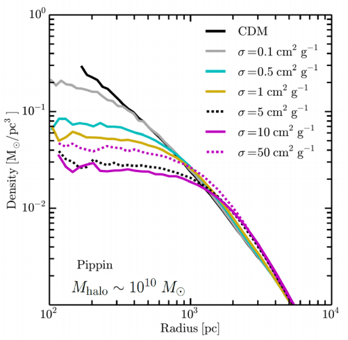
In figure 2, we can see the simulated density profiles of a dwarf galaxy given CDM (black), and various interaction cross sections for SIDM (colored). Simulations for cold dark matter halos exhibit a relatively constant $-1$ slope in log scale. As you approach the center of the galaxy, the density of the surrounding matter increases exponentially. With nothing preventing this collapse we are left with a sharply peaked central density, or what cosmologists refer to as a cusp.
If we keep everything in the simulation the same but introduce a dark matter self-interaction cross section $\sigma$, the two profiles look similar at radii larger than $1$ kpc. However, at smaller radii, the self-interactions generate a sort of “pressure”, preventing further collapse of the halo thereby forming a larger region of constant density at the center—or core—of the galaxy. Additionally, as is apparent from figure 2, the density profile of the dwarf galaxies is fairly resilient to the interaction cross section of SIDM we choose, which avoids any issues of fine-tuning.
Comparing the results of such observations of dwarf galaxy rotations with the simulations presented in figure 2, a telling picture emerges. Dark matter halos in dwarf galaxies form cores rather than cusps. To reiterate, these results come from DM-only simulations and despite their best agreement coming from dwarf galaxies, which are DM-dominated, there is still debate as to how resilient these results are to the introduction of processes involving baryonic matter.
The Missing Satellites Problem
Under the highest resolution simulations yet devised, we expect to see on the order of a few thousand subhalos with masses of $M_\text{peak} \gtrsim 10^7 M_\odot$.
Despite this, when analyzing data collected from observations only $\sim 50$ satellite galaxies with masses as low as $\sim 300 M_\odot$ have been detected. While it is likely more subhalos within the mass range expected will be found, it seems unlikely that enough can be found to completely resolve this tension.
\subsection{Self-interacting dark matter} Despite the fact that dark matter must interact only very weakly–if at all–with all forces other than gravity, provided that the dark matter particle is low mass, there is nothing that forbids self-interactions.
This is the foundation for self-interacting dark matter (SIDM). By assuming some self-interaction cross section for our dark matter particle, we can preserve the success of CDM on large scales, while mitigating some of the issues $\Lambda$CDM faces on small scales.
Interaction Cross-Sections
While there are differing accounts of the constraints on the interaction cross section of SIDM, observational constraints from the Bullet Cluster put the interaction cross section of dark matter at $\sigma/m \lesssim 1$ cm$^2$/g. This cross section is quite large by all accounts and would likely be large enough to resolve the core-cusp problem.
As explained earlier, many different dark matter candidates are allowed by the $\Lambda$CDM model. The same is true of SIDM, however with an added caveat. Since we require self-interactions, there must be both a SIDM particle and an associated mediator, both of which require new particles outside of the standard model.
In general, the force which governs the self-interactions is given as a Yukawa potential:
$$ V_Y(r) = \alpha ’ \frac{e^{-\mu r}}{r} $$
Here $\alpha$ is the coupling constant, $\mu$ is the mediator mass and $r$ is the distance to the particle. On possible SIDM mediator of the Yukawa potential could be a so-called dark photon which, unlike a typical photon, need not be massless. As the name implies, dark photons reside in a theoretical region know as the dark sector, outside the Standard Model of particle physics. The interaction cross section for self-interactions strongly depends on the ratio of mediator mass to particle mass.
This allows us to infer properties of the dark matter particle and its mediator, from constraints placed on the interaction cross section. This is very useful and has been used to constrain the ratio of masses based on observations of the Bullet Cluster (1E 0657-56).
Observational evidence
When it comes to actively analyzing dark matter, few regions in space hold as much promise as the Bullet Cluster. The Bullet Cluster is a high-velocity galaxy cluster merger.
As the two galaxy clusters merge, the gas which resides in the space around them collides at high velocities and begins to heat up, emitting x-rays. These x-rays can be observed and allow us to pinpoint the central mass of the baryonic matter. However, when we compare this with the distribution of total matter in the cluster, found through gravitational micro-lensing, we find a discrepancy. The mass distributions do not align. Not only does this point to the existence of dark matter, but it can be a valuable tool for determining constraints for the cross section of SIDM.
Additionally, by analyzing the shapes of the mass distributions of the galaxy clusters we can get some insight as to whether the dark matter underwent strong self-interactions, or if the dark matter halos acted as collisionless cold dark matter.
While the work our group is doing does not directly relate to the Bullet Cluster, it is one of the most promising places to look for observable evidence of SIDM.
Methods
In order to make predictions and build theories around SIDM, we rely on simulations. As mentioned earlier the only directly observable evidence for dark matter comes in the form of its gravitational influence.
While some attempts are being made to directly observe dark matter particles, most cosmologists rely on carefully analyzing the observable structure of galaxies, dark matter halos, and the Universe and comparing it with the structure as predicted by simulations.
Being able to vary the parameters for dark matter, define the initial conditions, then run the clock forward and analyze the resulting data is extremely powerful.
A promising application of this repeated simulation approach is simulating the time evolution of dark matter subhalos of the Milky Way. By generating initial conditions for dark matter subhalos and analyzing the simulation data as they interact with the Milky Way, we can better understand the effects self-interactions have on a subhalo’s evolution in the presence of its host.
This technique while effective is also extremely demanding in terms of compute hours. Simulating hundreds, thousands, or even millions of particles and their interactions on timescales on the order of the age of the universe is no easy task.
These simulations require lots of time on computer clusters (often referred to as supercomputers) to successfully run. Even on these clusters, we need to be extremely diligent in ensuring that the code responsible for the simulations is written efficiently.
Simulation Software
The analysis which follows builds on the work of Philip Hopkins, creator of GIZMO a fork of the earlier GADGET-2 N-body simulation suite written by Volker Springel. GIZMO is a massively parallel, multi-physics simulation suite, containing modules for hydrodynamics, fluid physics, star formation among others.
In 2010 code was added to the simulation suite of GADET-2 (and subsequently incorporated into GIZMO) to include self-interactions for dark matter simulations. It is this module that is the focus of several changes aimed at incorporating interactions between a simulated dark matter subhalo and its host.
Host-subhost interactions
As discussed earlier, dark matter halos are large regions of gravitationally bound dark matter, while subhalos are virialized clumps of dark matter contained within the larger host. Over time, as the subhalos orbit the center of the host halo, they undergo several effects which affect their mass distribution and density profiles.
Tidal Stripping
One such effect comes from tidal stripping. As the subhalo orbits ever closer to the central density of the host, its exterior begins to be stripped away by the gravitational pull of the host. This effect is more dramatic in the case of SIDM than it is for CDM. This is a direct result of the more cored density profiles SIDM creates. Since the central density of SIDM subhalos is larger and more diffuse than that of CDM, the matter at further radii from the center of the subhalo is bound less tightly and thus more easily stripped.
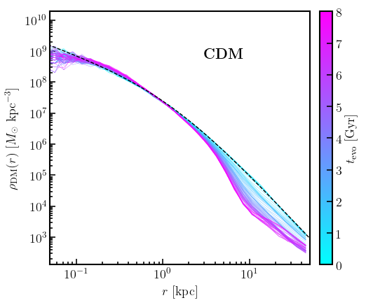
As we can see from figure 3, initially the dark matter subhalo is represented by an NFW profile. However as time increases, it’s density at around 10 Mpc is reduced, this is a result of tidal stripping. As more and more mass is stripped away from the subhalo, its density in the outer regions decreases.
Ram Pressure
Another effect on subhalo evolution is ram pressure. This is a sort of drag force resulting from the movement of a body through a medium. This drag is cause by the bulk motion of the particles in the two mediums as the move through one another. In the case of dark matter subhalos, ram pressure creates drag as the subhalo moves through the host halo’s background density.
Self-interactions
The self-interactions proposed by SIDM are not limited to the subhalo itself. As the subhalo falls into its host, the subhalo particles are free to interact with the particles in the host and visa versa. These interactions–while not currently included in most simulations–could affect the evolution of the subhalo.
While interactions between a DM subhalo and its host would have a minimal effect on the subhalo’s evolution at large distances, during infall the rate of host-sub interactions increases dramatically, which can cause changes in the subhalo’s evolution.
When considering the interactions between the host halo and the subhalo, there are two primary calculations which need to be considered, the probability of a given interaction, and the resulting momentum transfer.
Probability of interaction
First we need to calculate the probability that a given particle will interact with other particles in it’s neighborhood. GIZMO calculates this in the same way as presented in Kummer et al. 2017:
$$ \Gamma = \frac{\rho; \sigma;v_0}{m_\chi} $$
Here $\rho$ is the mass density of the DM background at the particle’s location, $\sigma$ is the cross section of the particle (this can be velocity dependent), $v_0$ is the particle velocity in the rest frame of the DM background, and $m_\chi$ is the dark matter mass.
At each timestep, GIZMO loops through all of the simulated particles and searches for neighbors close by which could possibly interact. For each neighbor, this probability is computed and compared against a random number generator to determine if an interaction has occurred.
Momentum transfer
Once an interaction is determined to have taken place, GIZMO applies a momentum transfer to the particle pair. The process is fairly straightforward as the collisions are elastic.
GIZMO calculates the angle at which the two particles scatter in a Monte Carlo process, assuming random angles in the center of mass frame of the collision, i.e. isotropic scattering. However, this is not completely accurate, in the particle collisions we expect the density of scattering angles to be sharply peaked in the forward direction.
A solution to the above issue should be implemented in future additions to the codebase but is not the focus of this research.
Simulating a live host
First, we could simulate the dark matter host halo in addition to the subhalo. To do this requires simulating all of the dark matter particles of the host halo regardless of if they ever interact with the subhalo. This method is quite simple, all that is required is to define the parameters of the host halo–in our case the Milky Way–and plug those parameters into GIZMO and allow it to manage the rest of the physics as usual. However, the simplicity of this approach comes at the steep price of computation time.
Since we are not interested in the evolution of the host halo, keeping track of all of its constituent particles throughout each timestep of the simulation would be extremely inefficient. The bulk of the mass of the halo is concentrated in the host, meaning there are far more simulated particles in the host than in our subhalo. The result is that most of our computational power will be spent calculating changes in particles which are of no interest to our research.
Using an analytic host
Another option is to represent the host halo as an analytic potential acting on the simulated subhalo. This certainly reduces unnecessary computation, since no particles in the host halo are resolved. However, the ground gained in terms of computational ease must be paid for in terms of the complexity of the method.
While before the probability of interaction could be computed directly. The solution for finding the probability of interaction for an analytic host is more involved.
Analytic host implementation
All credit for the below derivations is owed to Professor Manoj Kaplinghat. I have included them here for brevity, but these are not solutions I devised.
In order to calculate a probability of interaction for each particle, we will first define a priori the final form of the probability before defining the terms which are required to calculate it. For a particle at radius $r$ from the center of the analytic potential, the probability of interaction between it and the host halo is given as: $$ P = \Delta{t}, \rho(r) \mathcal{J}(r) $$
Here $P$ is the dimensionless probability, $\Delta t$ is the simulation timestep, and $\rho(r)$ is the density of the host halo at the particle’s position $r$ \footnote{We align the center of the simulation with the center of the host halo, thus $r_\text{host} = r_\text{particle}$}. The last quantity $\mathcal{J}(r)$ has units of $\frac{\text{Mpc}^3}{s\cdot M_\odot}$ and represents the weighted probability of interaction between the particle and the background velocity distribution of the host halo and can be written explicitly in the following form:
$$ \mathcal{J}(r) = \sum_{i} \mathcal{F}(v_{r,i},v_{t,i}|r) \int\mathrm{d}{v_{r}} \int\mathrm{d}{v_{t}} \int_{0}^{2\pi} \frac{\mathrm{d}{\phi}}{2\pi\Delta v_{r,i}\Delta v_{t,i}}, |\bm{v}-\bm{v}{s}| \times \sigma{m}(|\bm{v}-\bm{v}_{s}|) $$
We can replace the first term in the equation as $\mathcal{F}(v_{r,i},v_{t,i}|r) = 2 \pi v_t f(v_{r},v_{t},\phi | r)$. This is useful since $f$ is measured from results of N-body simulations. We can further simplify equation (6) by creating discrete bins in $v_r$ and $v_t$ again based on data from N-body simulations of the Milky Way. These represent the average radial and tangential velocities at a given radius. Since we are not working with discretized bins, we can simplify the integrals over $\mathrm{d}v_r$ and $\mathrm{d}v_t$ by replacing them with the bin sizes for the same quantities.
$$ \mathcal{J}(r) \simeq \sum_{i} 2 \pi v_t f(v_{r},v_{t},\phi | r) \Delta{v_{r,i}}\Delta{v_{t,i}}, \sum_{j} \int_{0}^{2\pi} \frac{\mathrm{d}{\phi}}{2\pi\Delta v_{r,i}\Delta v_{t,i}}, |\bm{v}-\bm{v}{s}| \times \sigma{m}(|\bm{v}-\bm{v}{s}|) \Big|{{v_{r,j},v_{t,j}}} $$
Since the end goal is to devise a method that is far less computationally intense than simulating the host halo, we want to calculate ahead of time as many values of the above equation as possible. By computing values that do not depend on the particle in question, and storing them in memory, we can avoid unnecessary repeated calculations. Recall that the host interaction probability is calculated once per particle per timestep, so efficiency is imperative. We will next define two parameters $A$ and $B$ whose purpose will become clear momentarily.
$$ A &= \sqrt{v^{2}+v_{s}^{2} - 2v_{r}v_{s,r}},\ B &= \frac{2v_{t}v_{s,t}}{v^{2}+v_{s}^{2}-2v_{r}v_{s,r} } $$ We can now input these parameters to the integral $\mathcal{I}$ in equation (7) \begin{equation} \mathcal{I} = \int_{0}^{2\pi} \frac{\mathrm{d}{\phi}}{2\pi}, g\left(A\sqrt{1+B\cos(\phi-\phi_{0})}\right) \end{equation} Here $g(x) = x\cdot \sigma_0/(1+x^4)$ and the bounds on $A$ and $B$ are $A\geq 0$ and $0\leq B \leq 1$. After a some changes of variables, integration bounds, and variable substitutions, we arrive at an equation for $\mathcal{I}$ as follows: \begin{equation} \mathcal{I} = g\left(A\right) \frac{1}{\pi} \int_{1-B}^{1+B} \mathrm{d}{\xi}, \frac{g(A\sqrt{\xi})}{g(A)} \left[ (1+B-\xi)(\xi-(1-B)) \right]^{-\tfrac{1}{2}} \end{equation}
Once this integral is calculated, we can plug it back into equation (7) and solve for $\mathcal{J}(r)$. Once this is solved we can take the ratio of the ith bin result of $\mathcal{J}(r)$ and the sum of $\mathcal{J}(r)$ across all bins, and plug this back into equation (5) to solve for the probability of interaction for a given particle. The computation of this integral is likely the most resource-intensive, this is why we choose to calculate it once at runtime, rather than at each timestep. Calculating it ahead of time and storing it in a 2D interpolation grid is the focus of section
Results and Discussion
GIZMO is written in the coding language C. It uses libraries such as the GNU science library (GSL), fast Fourier transform (FFTW), and MPI for parallelization. When adding functionality to the code to account for the host to subhalo interactions, it is important to preserve the original functionality of the code and extend it. To facilitate this we add a flag to GIZMO’s configuration that when toggled in the Config.sh file, will enable host-subhalo interactions. However, when the flag is not enabled, the code will act identically to stock GIZMO with no modifications. This is achieved by wrapping all-new functions, variables, loops, etc. within compile-time preprocessor directives which check to ensure the flag is toggled in the configuration file before including the content in the compiled binary. These preprocessor directives have been omitted from the included code for simplicity, but assume for all code blocks described below, they are only active given the flag in Config.sh.
2D Interpolation of $I$
One of the most computationally demanding aspects of this method of calculating host-subhalo interactions is the calculation of the integral in equation (11). We use a numerical integration approach that converges on a value within some error of the true value. This method is quite fast but it is still demanding when considering the sheer number of times it would need to be computed. So rather than calculate this integral for each particle at each timestep of the simulation, the integral is instead computed several hundred times as a function of parameters $A$ and $B$ then stored in an interpolation grid at runtime for use throughout the simulation.
Required functions
In order to calculate all the integral values and store them in a grid, we first need to define the function $g(x)$ which is referenced in the integrand. Since we only want to apply interaction velocity scaling at the request of the user, we start by checking for the velocity scale flag and if it is toggled, we apply the scaling. The function then returns a double based on the definition of $g(x)$ given in the methods section.
double g_func(double x) {
    if(All.DM_InteractionVelocityScale>0) {double x = x/All.DM_InteractionVelocityScale;}
    return x*All.DM_InteractionCrossSection/(1 + x*x*x*x);
}
We next define a function representing the closed form of the integrand, which will be used to calculate the numerical integral. The below code defines a function integrand which takes two arguments, the value of the variable being integrated over, as well as a void pointer, responsible for storing all the other constants, and parameters that need to be passed to the function to recreate the integrand in equation (11).
When the function is called, it casts the void pointer to a pointer of type int_params, a structure of two doubles one storing $A$ the other $B$. It then returns the result of the integrand in equation 11, using the correct values of $A$ and $B$ stored in the pointer $p$. The function also makes references to our previous definition of g_func.
double integrand(double x, void *p) {
    struct int_params *params = (struct int_params *)p;
    return g_func(params->A*sqrt(x))/g_func(params->A) * 1.0/sqrt((1 + params->B - x)*(x + params->B - 1));
}
Initializing the Interpolation Grid
Having defined both of the relevant functions of the integral $\mathcal{I}$, we can now create our 2D interpolation grid. For this, we use GSL’s gsl_interp2d library. We begin by allocation memory for the set of points $A$ and $B$ which define the shape and number of computed values in the grid along with memory for the points $\mathcal{I}$. The number of points $\mathcal{I}$ is the product of the length of the vector of $A$ points and the length of the vector of $B$ points. We now want to define our set of $A$ and $B$ points by populating the array with a number of evenly spaced points equal to $A_\text{res}$ and $B_\text{res}$ for $A_\text{min} \leq A \leq A_\text{max}$ and $B_\text{min} \leq B \leq B_\text{max}$ respectively. Here the limits of $B$ are defined unilaterally as $B_\text{min} = 0$ and $B_\text{max} = 1$, while the limits of $A$ are defined with respect to the velocity interaction scale set by the user.
The function then allocates memory for the grid, storing the results in the globally accessible. To improve the speed at which results are queried from the grid, we define two acceleration pointers for $A$ and $B$ which keep track of the previous $A$ and $B$ parameters requested to be able to more quickly provide responses in the event we request an interpolated value close to another previously requested one.
After correctly formatting our previously defined functions and structures in a way to make them usable by the GSL library, we enter a nested for loop, which iterates over all combinations of $A$’s and $B$’s within the set of points A_pts and B_pts. For each point $(A, B)$ we evaluate the numerical integral to within an acceptable relative error ($1e-4$) using the non-adaptive Gauss-Kronrod integration method within the GSL library. The function then stores this value times $\frac{g(A)}{\pi}$ into the corresponding grid point based on $A$ and $B$. Once the function has looped through all the $A$ and $B$ points, it then initializes the grid with all the correct values and dimensions. This function is called only once during the startup of the simulation and can be queried at any time to produce an accurate estimate of the value of the integral at the given parameters, without substantially affecting the computation time, since we are checking an interpolated value rather than calculating an integral.
void init_interp_grid()
{
A_pts = malloc(A_res*sizeof(double));
B_pts = malloc(B_res*sizeof(double));
I_pts = malloc(A_res*B_res*sizeof(double));
for(int i = 0; i < A_res; i++) {*(A_pts + i) = i*((double)A_max/A_res);}
for(int j = 0; j < B_res; j++) {*(B_pts + j) = j*((double)B_max/B_res);}
sh_interp2d_integral = gsl_interp2d_alloc(gsl_interp2d_bilinear, A_res, B_res);
A_interp_acc = gsl_interp_accel_alloc();
B_interp_acc = gsl_interp_accel_alloc();
gsl_function F;
F.function = &integrand;
struct int_params params;
for(size_t i = 1; i < A_res; i++) {
for(size_t j = 1; j < B_res; j++) {
params.A = *(A_pts + i);
params.B = *(B_pts + j);
F.params = (void *)¶ms;
size_t neval;
double result, error;
double lbound = 1 - *(B_pts + j);
double ubound = 1 + *(B_pts + j);
int code = gsl_integration_qng(&F, lbound, ubound, epsabs, epsrel, &result, &error, &neval);
gsl_interp2d_set(sh_interp2d_integral, I_pts, i, j, g_func(params.A)*result/M_PI);
}
}
gsl_interp2d_init(sh_interp2d_integral, A_pts, B_pts, I_pts, A_res, B_res);
}
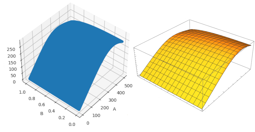
As mentioned before the above code produces a 3D grid of values. In order to verify that this function produces a correct grid of values, it was checked the same grid produced in Mathematica. The results can be seen in the figure below. The side-by-side comparison shows very good agreement between the two methods so we can proceed with relative confidence.
Interpolation lookup
Now that we have an interpolation grid we need a new function to act as a lookup function. It takes two arguments, $A$ and $B$, and returns a value of the integral $\mathcal{I}$ regardless of the parameters passed to it. This is important since querying the GSL interpolation grid for values outside the bounds for $A$ and $B$ will result in an error, potentially crashing the simulation and corrupting the data collected. To avoid this, our new lookup function will take any values of $A$ and $B$ and return an accurate result.
It first checks if the point passed lays within the interpolation grid produced in the previous section. If the point is within the grid we simply query the grid for the result and return the given value. Next, if the point $(A,B)$ is within bounds of $B$ but below the minimum value of $A$, we can calculate an analytic solution to the function. This is because in the limit where $A$ is quite low, its dependence drops out of equation (11) and we are left with an integral which can be solved analytically. Namely:
$$ \mathcal{I} = g\left(A\right) \frac{1}{\pi} \int_{1-B}^{1+B} \sqrt{\xi}\left[ (1+B-\xi)(\xi-(1-B)) \right]^{-\tfrac{1}{2}};\mathrm{d}{\xi} $$
The calculation of this analytic integral is to be added at a later date. Finally, if the points $A$ and $B$ passed to the function lay outside the limits of $B$ or above the upper bound on $A$, we return 0. This corresponds to zero probability of interaction. Points outside the bounds on $B$ represent non-physical values, and should not be considered, while values above the upper limit of $A$ are still physical, they are well approximated by zero.
double integral_lookup(double A, double B) {
    if((A > A_min && A < A_max ) && (B > B_min && B < B_max )) {
        return gsl_interp2d_eval(sh_interp2d_integral, A_pts, B_pts, I_pts, A, B, A_interp_acc, B_interp_acc);
    }else if((B > B_min && B < B_max ) && A <= A_min) {
    /* Analytic solution to be added. */
    }else{return 0;}
}
Probability of Interaction
To calculate the probability of interaction between a given particle and the host halo we need to know some information about the region of the host halo local to the particle in question. Namely, we need to know the host background density. To do this a function has been included which takes the particle radius\footnote{See footnote 1} as an argument and returns the NFW density of the Milky Way at the point $r$.
double NFW_density_calc(double r) {
    double x=r/SH_Rs;
    return SH_p_const/(x*(1+x)*(1+x));
}
Given all the above functions we can now calculate the probability of interaction between a given subhalo particle and its analytic host halo. The function begins by taking in as arguments the particle mass, the particle position $r$, the particle velocity $V$ and position Pos, and the timestep $dt$.
To calculate the probability of interaction we follow closely with the procedure laid out in section 2.3. We begin by calculating the magnitude of the particle’s velocity converting to physical units. We next generate angles $\theta$ and $\phi$ from the particle position to be used later in the calculation of the radial and tangential velocities of the particle. Next, the function pulls the values of vr and vt (the radial and tangential velocity of the background host halo) from tables based on the particle position. After calculating the magnitude of the background halo velocity, we can get values for $A$ and $B$, which are passed to our integral lookup function, before calculating the background density from particle position and then multiplying the product together to generate a dimensionless probability of the form given in equation (5).
There are a few aspects of the code which have not yet been implemented. While the data has been collected we have not yet incorporated the velocity profiles of the Milky Way into a function that calculates based on the particle’s position. Additionally, as seen in section 4, there is a preliminary function written up for the calculation of the first term in equation (7), named “dagger” in the probability function, but it has not yet been verified.
double prob_of_host_interaction(double mass, double r, double V[3], double Pos[3], double dt)
{
    double Vmag = sqrt(V[0]*V[0]+V[1]*V[1]+V[2]*V[2]) / All.cf_atime;
    double theta = acos(Pos[2]/r), phi = atan(Pos[1]/Pos[0]);
    double vs2 = Vmag*Vmag;
    double vsr = V[0]*sin(theta)*cos(phi) + cos(theta)*(V[1]*sin(phi) + V[2]);
    double vst = sqrt((V[0]*cos(theta)*cos(phi) + V[1]*cos(theta)*sin(phi) - V[2]*sin(theta))*(V[0]*cos(theta)*cos(phi) + V[1]*cos(theta)*sin(phi) - V[2]*sin(theta)) + (V[0]*sin(phi)-V[1]*cos(phi))*(V[0]*sin(phi)-V[1]*cos(phi)));
    double vr = 0, vt = 0;
    double v2 = vr*vr + vt*vt;
    double A = sqrt(v2 + vs2 -2*vr*vsr), B = 2*vt*vst/A;
    double I_val = integral_lookup(A, B);
    double dagger = 0;
    double NFW_rho = NFW_density_calc(r) * All.cf_a3inv;
    double units = UNIT_SURFDEN_IN_CGS;
    if(All.DM_InteractionVelocityScale>0) {double x=Vmag/All.DM_InteractionVelocityScale;}
    return dt * NFW_rho * dagger * I_val * units;
}
Momentum Transfer
The other half of the method relies on being able to accurately apply the momentum kick to the subhalo particle once we have determined an interaction to have occurred. Unlike interactions within the subhalo, for interactions between the subhalo and the host, we are only interested in the momentum transfer to the subhalo particle. Since the host is represented analytically, we are not gathering any information on changes to it, and thus we can ignore the momentum transfer to the host. To calculate the momentum transfer for the subhalo particle, we do not need to create a new function but rather we need to be clever about the parameters passed to the existing kick calculation built into GIZMO.
void calculate_interact_kick(double dV[3], double kick[3], double m)
{
    double dVmag = (1-All.DM_DissipationFactor)*sqrt(dV[0]*dV[0]+dV[1]*dV[1]+dV[2]*dV[2]);
    if(dVmag<0) {dVmag=0;}
    if(All.DM_KickPerCollision>0) {double v0=All.DM_KickPerCollision; dVmag=sqrt(dVmag*dVmag+v0*v0);}
    double cos_theta = 2.0*gsl_rng_uniform(random_generator)-1.0, sin_theta = sqrt(1.-cos_theta*cos_theta), phi = gsl_rng_uniform(random_generator)*2.0*M_PI;
    kick[0] = 0.5*(dV[0] + dVmag*sin_theta*cos(phi));
    kick[1] = 0.5*(dV[1] + dVmag*sin_theta*sin(phi));
    kick[2] = 0.5*(dV[2] + dVmag*cos_theta);
}
This function–already defined in GIZMO–takes in a 3-vector of the relative velocity between it and its interaction partner, the particle mass, and an empty 3-vector in which to store the velocity change in each Cartesian coordinate. It then calculated the magnitude of the relative velocity, applies velocity dependent scaling if applicable, then recreates isotropic scattering by randomly selecting scattering angles, before finally converting these into velocity boosts in each Cartesian coordinate.
For the purposes of an analytic host, we already needed to calculate the velocity in spherical coordinates of the region of the host halo background with which the particle interacted. To calculate apply this towards the calculation of kick, we need to transform these to Cartesian coordinates, calculate the relative velocity between the patch of background and the particle, and pass that through to the above function to generate the kick vector.
Timestep loop
The final aspect of the code is to incorporate all the above functions into the codebase in the correct locations and make calls to them where necessary. As described in 2.2.4 GIZMO has a neighbor search loop built into its code. The additional calculation of the probability of interaction with the host and the calculation of the kick–provided an interaction occurs–are both included just prior to the search for neighbors. At each timestep GIZMO loops through all the particles in the simulation, checks to see if a given particle has an interaction on that timestep with the host, provides a boost if it does, then proceeds to search for nearby SIDM particles within the subhalo to interact with.
if( ((1 << local.Type) & (DM_SIDM)))
{
    double r = sqrt(local.Pos[0]*local.Pos[0] + local.Pos[1]*local.Pos[1] + local.Pos[2]*local.Pos[2]);
    double prob_host = prob_of_host_interaction(local.Mass, r, kernel.h_i, local.Vel, local.Pos, local.dtime);
    if(prob_host > 0.2) {out.dtime_sidm = DMIN(out.dtime_sidm, local.dtime*(0.2/prob_host));}
    if (gsl_rng_uniform(random_generator) < prob_host)
    {
        double kick[3]; calculate_interact_kick(local.Vel, kick, local.Mass);
        int i; for(i = 0; i<3; i++) {
            #pragma omp atomic
            local.Vel[i] += kick[i];
        }
    }
}
Future Work
In several places in section 3, there calls for future work. While lots of progress has been made on the modifications to GIZMO the project is not yet complete. Most of the necessary additions are minor, one in particular (for which an untested implementation is included below) is large. The project will continue, with my graduate student mentor taking over for the remainder of the changes. Several weeks were spent bringing him up to speed on the status of the project, going over aspects of the code that may be confusing, extensively documenting the changes in the form of official documentation as well as code comments, and providing guidance on working with the code, pushing changes to the git repository and programming in C.
Summation of $f$ in velocity bins
To calculate the first summation of equation (7), we need to construct bins in radial and tangential velocity for the host and calculate the value of $f$ in each bin. Since this portion has no dependence on the particle in question, we can compute it once at runtime, store it in memory, and access it globally through a list of values.
In the function scriptF, we will take in as arguments the radius $r$ and the radial bin number, $r$_bin\footnote{It is possible to take in either just the radius or the bin and convert one to the other. This however has not yet been implemented in any way.}. We then loop through the number of velocity bins and store the value of the resulting formula in each cell of the array under index $i$\footnote{We will define the numbers of bins in r and in tangential and radial velocities in a header file rather than on lines 2 and 3. This also goes for the variables fF and sum_fF, they will be declared in a globally available header file, then initialized in this function’s loops.}. The function then enters a nested loop which iterates over both the radial bins and the velocity bins, and sums over the radial velocity bins and stores them in an array based on radius sum_fF. This vector can not be called in the probability of interaction with host function and is only computed once, and thus has a minimal computational impact.
$$ 2 \pi v_{t,i} f(v_{r},v_{t},\phi | r) \Delta{v_{r,i}}\Delta{v_{t,i}} $$
double scriptF(double r, int r_bin){
    const size_t num_bins = 15;
    const size_t num_rbins = 14;

    double fF[num_rbins][num_bins];
    for(int i; i < num_bins; i++) {
        double dagger = 2*M_PI*vel_t_bins[i]*fv_r[i][rad]*fv_t[i][rad]*(vel_t_bins[i+1]-vel_t_bins[i])*(vel_r_bins[i+1]-vel_r_bins[i]);
        fF[r_bin][i] = dagger;
    }

    sum_fF[num_rbins];
    for(int i; i < num_rbins; i++) {
        double sum_value = 0;
        for(int j; j < num_bins; j++) {
            sum_value += fF[i][j];
        }
        sum_fF[i] = sum_value;
    }
}
Anisotropic Scattering
As mentioned in section 2.2.5, we briefly mention that at present GIZMO assumes all scattering with SIDM occurs randomly, with equal probability, at all angles. This is a common example of Monte Carlo simulations which rely on large numbers of events to be able to randomize the parameters of the simulated events within a given range. Here were are randomizing the angle along the interval $ (0,2\pi) $. However, the code should take into consideration the fact that the possible angles of scattering are sharply peaked in the forward direction. When two particles collide, it is far more likely that they interact and scatter forward, than it is they scatter backward, or orthogonally to the CM frame. This correction will likely be minor and shouldn’t be prohibitively difficult to implement at a later date.
Testing
While individual aspects of the code have been tested, no testing has yet been run on the complete method. Once the remainder of the changes have been implemented into the code, extensive testing and data analysis should be done, under close supervision from an expert in the field, to ensure that no mistakes were made and that the code is capturing true physics. Given that the group has access to several computer clusters and has a sizeable allotment of time on those clusters, this should be a fairly straightforward task, and one that I wish I could be a part of.
Conclusion
Modifications to the GIZMO simulation suite were made, with over 60 code commits in total. These changes vary from minor corrections to existing comments, to two additional configurations for computer clusters, to large methods incorporating data to calculate particle interactions. We devise a new method for calculating the probability of interactions between a simulated subhalo and its analytic host. From this probability, we can quickly estimate the likelihood that a given particle at a given timestep would interact with a particle in the host halo, then use information about the particle’s position and the properties of the host halo to calculate the momentum change of the particle in the subhalo.
The effects of host-subhalo interactions are not small, during infall subhalos can experience large amounts of ram pressure as a result of their motion through the host halo’s background density. This ram pressure is likely to come with large numbers of interactions between the particles of the subhalo and those of the host. These results could alter the time evolution of subhalos in simulations and could better approximate their true evolution, provided the SIDM model continues to solve issues other dark matter candidates cannot.
While the changes have not been tested in their entirety, they have been individually tested, check for errors, and where possible results have been analyzed. Preliminary results–prior to the incorporation of much of the code–showed an increase in computation time of approximately $ 20% $. The expected increase in computation time with all of the code in place is much higher, but this suggests it will likely still be substantially more efficient than simulating the entire host halo with live particles throughout the simulation.